Bart H. McGuyer
Visual shortcuts for Lewin's circuit paradox
TLDR: Some figures and shortcuts to help explain a fun classroom demo involving circuits and electromotive force.
One of my favorite classroom demonstrations is “Lewin’s circuit paradox.” This demo typically shows two voltmeters giving different readings despite having their leads connected to the same two points on a circuit. (See Ref. 1 for a video.) Though this difference is surprising, there isn't an actual paradox. Instead, the demo cleverly highlights how the contribution from induced electromagnetic force (or emf) varies with the exact route taken by the leads of each voltmeter. If you want to dig deep into the details, I recommend Refs. 2—5. If you're searching for a visual approach, this Note offers a few figures and shortcuts to help explain the demo.
Control circuit:
To begin, let's start with a "control" circuit that has no emf and no apparent paradox. Fig. 1 shows an ideal circuit made of two identical resistors of finite, positive resistance \(R\) connected in parallel with a signal generator. As sketched, the resistors form a closed loop. Two ideal voltmeters, labeled by their readings \(V_1\) and \(V_2\), connect to this loop at its top (point A) and its bottom (point B). Note that their leads connect with the same polarity: red to A, and blue to B.
Taking a look at Fig. 1, do you think the two voltmeters should give identical readings?
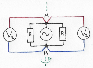
Figure 1: Warmup with a "control" circuit.
The answer is yes, the two readings should be identical: \(V_1 = V_2\). (This assumes Fig. 1 is ideal: If you build a real circuit, the readings will likely deviate a bit because of practical details that we've neglected.)
Visual shortcuts for the control circuit:
Here're two shortcuts to help get to this answer:
1st shortcut: Notice that any currents in the resistors must be equal and must flow in the same vertical direction: either both up or both down. Therefore, the voltages across those resistors, and thus measured by the voltmeters, will be identical.
2nd shortcut: Notice a symmetry about the line A-B, as hinted by the green dashed line and green arrow [4]. Either reflecting or rotating by 180 degrees about that line swaps the voltmeter positions but changes nothing else, again requiring equal readings.
Lewin's circuit paradox:
With Fig. 1 handled, I think we're ready! Fig. 2 shows an ideal version of Lewin's circuit paradox. Its form comes from replacing the signal generator in Fig. 1 with a source of emf. In Fig. 2, the shaded circle is the emf source, and it represents a cross section of an ideal, infinite-length solenoid inductor with a uniform, time-varying current. This solenoid provides a time-varying magnetic flux within the shaded region that induces an emf in the loop. (In a real circuit, a slow triangle or ramp waveform might be convenient for the current to help compare simultaneous readings.)
Taking a look at Fig. 2, do you think the two voltmeters should give identical readings?
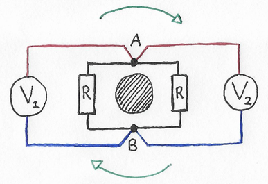
Figure 2: Lewin's circuit paradox (ideal version).
The answer is no. While the two readings will still be equal in magnitude, they'll now be opposite in sign: \(V_1 = -V_2\). (If you build a real circuit with sinusoidal current, you'll need either an oscilloscope or sign/phase-sensitive voltmeters to see this difference.)
Visual shortcuts for Lewin's circuit paradox:
Here are four shortcuts to help get to this answer:
1st shortcut (revisited): Notice that the currents in the resistors, while still equal, must now flow in opposite vertical directions: one up and the other down. (The 3rd shortcut will help show this.) Thus the voltages across those resistors will be equal except in sign.
2nd shortcut (revisited): Notice that, because of the change in current direction, the circuit is now symmetric for rotations about the emf source, as hinted by the green arrows [4]. Rotating by 180 degrees swaps the voltmeter positions while reversing their polarities, but changes nothing else, again requiring equal but opposite readings.
3rd shortcut: In the next section, Figs. 3-5 show how to simplify the circuit by replacing the emf source with an equivalent signal generator.
4th shortcut: In the final section below, Figs. 6 & 7 extend this to consider what happens when a voltmeter moves from one side to the other, showing why there is a difference between their readings.
3rd shortcut details:
Let's make this circuit easier to interpret by removing the emf source. Fig. 3 shows the first step, which is to pull the emf source out sideways. Doing this splits point B into points B\(_1\) & B\(_2\):
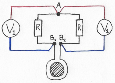
Figure 3: Lewins's circuit paradox with the emf source outside the loop.
Moving the source outside the loop takes most—but not all—of its emf with it. To remove all remaining emf, let's adjust the two ideal wires connecting points B\(_1\) & B\(_2\) to the source so that there's no area between them. (For a real circuit, consider braiding those wires and moving the source far enough away to suppress stray fields at the loop.) At this point, the circuit no longer has any induced emf from the source within the region around the loop and voltmeters, but otherwise is unchanged. That is, the readings are the same as before, and they'll stay unchanged if we next replace the source with an equivalent signal generator connected to points B\(_1\) & B\(_2\):
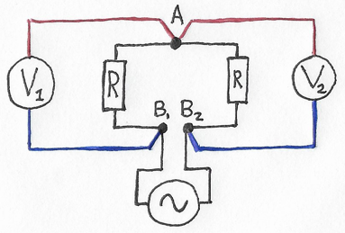
Figure 4: Lewins's circuit paradox after replacing the emf source with an equivalent signal generator.
With these changes, note that the circuit of Fig. 4 resembles that of Fig. 1, but with the signal generator moved from connecting A & B to connecting B\(_1\) & B\(_2\). Re-arranging gives Fig. 5 below, which should be a little easier to interpret: Here, the currents in the resistors must flow in the same direction: either both left or both right. However, the voltmeters are connected in opposing directions, so give opposite readings.

Figure 5: Simpler layout of the circuit in Fig. 4.
4th shortcut details:
Finally, let's consider what happens if we move one voltmeter from its side to the other side, just as you could do during a real demo. If the readings differ, then the moving voltmeter's reading should change and, eventually, match the other meter's reading. For clarity, let's leave the original voltmeters as is, and add a third voltmeter in the middle, labeled by its reading \(V_3\). Doing this splits the emf source into two subsources about \(V_3\), shown below by shaded semicircles. Following the 3rd shortcut, let's go ahead and pull these subsources out by trisecting point B.
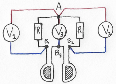
Figure 6: Lewins's circuit paradox with a third voltmeter. The emf source is outside the loop, and split into left and right subsources.
During a demo, when you move a voltmeter from one side to the other, what changes is the division of the flux from the source between the "left" and "right" sides of that voltmeter (and its leads). This is mimicked here by dividing the flux between the two subsources. What doesn't change is the total flux produced by the source, which here means that the total flux produced by those subsources must sum to a constant. Otherwise, the readings \(V_1\) and \(V_2\) won't stay constant.
Therefore, to simulate moving the new voltmeter \(\left(V_3\right)\), let's keep the total flux produced by the subsources constant, but alter how this flux is divided between them. Then, to start with the voltmeter \(V_3\) on the same side as \(V_1\), turn off the left subsource, so that all emf comes from the right subsource. Finally, to simulate moving \(V_3\) over to the same side as \(V_2\), gradually turn off the right subsource, until all of the emf comes from the left subsource.
To see how the reading \(V_3\) changes while its voltmeter moves, let's convert the emf sources into equivalent signal generators, just like in the 3rd shortcut:
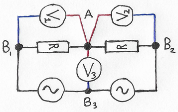
Figure 7: Equivalent circuit for Fig. 6 after replacing the emf subsources with equivalent signal generators and simplifying the layout.
With these changes, note how the circuit of Fig. 7 now resembles that of Fig. 5, but with the signal generator split by the new voltmeter. To simulate moving \(V_3\), we now need to keep the sum of the two generators constant, but alter how this signal is divided between the left and right generators. To place the voltmeter \(V_3\) on the same side as \(V_1\), turn off the left generator, so that all the signal comes from the right generator. Then, to move \(V_3\) over to the same side as \(V_2\), gradually turn off the right generator, until the left generator provides all the signal. Thus the total signal changes from being generated on the right of \(V_3\) to being on its left, explaining the sign change. This also shows that once the voltmeter is exactly half way between both sides, such that the two generators give matching signals, then \(V_3 = 0\). (For an explanation using transformers, with motion adding or removing secondary windings, see Ref. [3].)
Alternatively, if adjusting the two generator signals is hard to imagine, instead consider splitting the original generator into many more subgenerators in series, say N = 10 of them, instead of just N = 2 as used in Fig. 7. Then, if each subgenerator outputs an equal signal, we could simulate motion by moving \(B_3\) to connect between different pairs of neighboring subgenerators, instead of by adjusting any signals. Doing this, you could imagine, in a stop-motion fashion, that the voltmeter \(V_3\) effectively rotates about its connection to point A, while its connection \(B_3\) moves from one side of all the subgenerators to the other, sort of like the moving tap in a variac or a variable resistor. As it moves, \(V_3\) transitions from being in parallel with one and then with the other of the original voltmeters.
While none of these ideas are new, hopefully this Note presents them in a way to help explain this fun demo. I'm grateful to Ben Olsen, Brian Patton, and Justin Brown for asking whether or not \(V_3\) is zero at the midpoint, which led to this Note.
References- [1] Here's a video of a Lewin's circuit paradox demo:
"Demo 12304: Nonconservative Electric Field." YouTube, uploaded by "Caltech's Feyman Lecture Hall," Apr 1, 2020.
Link: https://www.youtube.com/watch?v=eKJDylS3GqE - [2] Here's a video of Prof. Lewin himself explaining the demo:
"Solutions to Problem #93 - 2 Voltmeters." YouTube, uploaded by "Lectures by Walter Lewin. They will make you ♥ Physics," Sep 9, 2020.
Link: https://www.youtube.com/watch?v=SuKJxhOTDE4 - [3] For a deep dive, I highly recommend this:
Kirk T. McDonald, "Lewin's Circuit Paradox," from Physics Examples and other Pedagogical Diversions, Nov 14, 2018.
Available online: http://kirkmcd.princeton.edu/examples/lewin.pdf - [4] Figs. 1 and 2 and the symmetry shortcut were adapted from this:
B. H. McGuyer, "Symmetry and Voltmeters," Am. J. Phys. 80, 101 (2012). ( Link to free PDF ) - [5] For many more pedagogical treatments of Lewin's circuit paradox, see the references listed within Refs. [3] & [4].
(May 2025)
© , bartmcguyer.com